
A Brief Introduction to R-tree
Motivation
My day job involves dealing with processing Euclidean and geospatial data. One of the most common task is to find the nearest neighbors for any given point.
Although the task can be approached from a brute force angle, it quickly becomes unfeasible as the time complexity grows exponentially with input size. A more efficient algorithm is needed to handle the queries in a reasonable amount of time.
R-Tree
Fortunately, minds more brilliant than mine had already came up with good solutions. In 1984, Antonin Guttman invented the R-tree, a data structure frequently used for spatial access methods. This data structure is particularly efficient for indexing multi-dimensional information such as geographical coordinates, rectangles and polygons [1].
How It Works
Unlike structures that uses a 1-dimensional ordering of values (B-trees and ISAM), R-tree groups nearby objects and represent them with their minimum bounding rectangle in the higher level of the tree [1]. This is better illustrated with the diagram below.
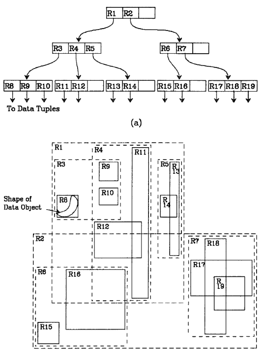
Figure 1. R-tree representation shown in Antonin Guttman's original paper [2].
For example, boxes R8, R9 and R10 are grouped together and are represented by higher level bounding box R3. In R-tree form, R8, R9 and R10 are child nodes of the parent node R3. Similarly, R3, R4 and R5 are bounded by R1, and hence are child nodes of R1.
Since all child nodes lie within their parent node, a query that does not intersect the parent node cannot intersect with any of the child node. This drastically reduces the search space from O(n2) to O(logMn) in the average case and O(n) in the worst case.
Applications
For the points and geometries that I work with, filtering overlaps is a common procedure. In the Euclidean space, this means applying intersection over union algorithms to the detection boxes.
However, there are edge cases that IOU filters cannot handle. For example, two adjacent bounding boxes are on the same object, but do not overlap. Another example involves overlapping boxes that does not meet the IOU threshold.
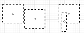
Figure 2. Edge cases encountered during IOU
Using R-tree on the points, instead of the boxes, allows for neighbor points and/or geometries to be queried without using the naive approach.
Code
Boost has a good implementation of R-tree that I used for my problem.
First, the R-tree is initialized. Boost’s R-tree comes with various initialization strategies that allow users to use different balancing algorithms (quadratic, linear, etc.), as well as setting the minimum and maximum amount of nodes.
Afterwards, the points are inserted into the R-tree. The tree is self-balancing such that child nodes of a parent node do not intersect with the child nodes of other parent nodes.
Boost comes with a suite of commands that can make complex queries more terse. To be specific, rtree.query is applied on a lambda function that compares point distance against a threshold.
void RTreeFilter(points points)
{
    bgi::rtree< value, bgi::quadratic<16> > rtree; //Initialize the R-tree data structure
    int id = 1;
    std::vector<int> indices;
    int filterThres = 50;

    for (int i = 0; i < points.size(); i++) // Populate the R-tree with nodes
    {
        int centerX = points[i][0];
        int centerY = points[i][1];
        point p = point(centerX, centerY);
        rtree.insert(std::make_pair(p, id));
        indices.push_back(id);
        id++;
    }

    for (int i = 0; i < points.size(); i++) // Find the nearest neighbors using R-tree
    {
        int centerX = points[i][0];
        int centerY = points[i][1];

        std::vector<value> returned_values;
        point sought = point(centerX, centerY);

        rtree.query(bgi::satisfies([&](value const& v) { return bg::distance(v.first, sought) < filterThres; }),
            std::back_inserter(returned_values));

        for(int distance : returned_values)
        {
            // Do something with the neighbors
        }

    }
}
Performance
Benchmarking for the naive approach vs the R-tree approach is shown below.
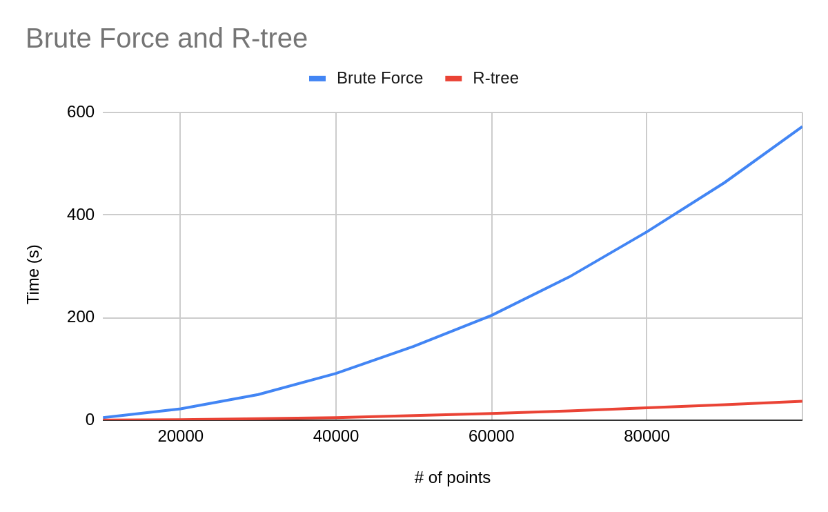
Figure 3. Benchmark comparison between brute force and R-tree spatial query
The benchmark program is written in C++. Test data points are generated within an arbitrary boundary of 5000px by 5000px. The number of input data is increased from 10000 to 100000, with an interval of 10000.
Right from the start, the R-tree algorithm outperforms the brute force approach and hence is the clear winner.
Other Applications
The R-tree algorithm is commonly used by GIS libraries operating on geospatial datasets. For instance, a user might want to find the closest coffee shops within a 20km radius of a given point. This can be easily achieved by using Geopandas and a few line of Python code.
Fun fact: Geopandas uses R-tree to implement the geospatial intersection and queries.
Summary
The post gives a brief explanation of R-tree and its use case. Thanks for reading, and look out for more future posts.
References
[1] https://en.wikipedia.org/wiki/R-tree
[2] http://www-db.deis.unibo.it/courses/SI-LS/papers/Gut84.pdf